Simple outlook inbox analysis using R

Emails from eBay members asking questions come through as randomstring@members.ebay.com which can make them hard to count as a group
The following R script re-codes them so they can be counted.

install.packages("plyr")
library(plyr)

setwd("/home/mike/Desktop")
dir()
inbox<-read.csv("inbox.TXT", sep="\t")
names(inbox)

inbox$EADD <- ifelse(grepl("members.ebay.co.uk",inbox$From...Address.), 
                      "members.ebay.co.uk" , 
                      c(as.character(inbox$From...Address.)))   

str(inbox)

f <- ddply(inbox,c("EADD"),summarize,N=length(EADD))
plot(f$N)
head(f[order(-f$N),])
str(f)

Once you've identified the biggest culprits, make a rule to move or delete them from your email.
Recoding a factor

When you have N levels of a factor but you would like M (M < N) you need to recode the data set.

when you run str(df) you get an idea that factors are numbered in any vetor or data frame.

We need to use a command to recode the levels. The command you use is ‘levels’:

levels(df$factor)[c(2,4,6,7)] = "Horse Whispering"

Which means: Take levels that have the internal numberings of 2,4,6,7 and convert them to being “Horse Whispering”.
To recode the rest you need to find the internal numbering of the new levels for the df:

levels(df$factor)

because the levels that were formally 2,4,6 and 7 have now been recoded into a single value and you’ll have to adjust the integers that you are using every time you run the command.

Continue on until all the necessary coding has been completed.

To make sure you have recoded properly you should make a copy of the first factor and recode the copy rather than the original. That way you can compare new and old later:

table(df$OrigFactor , df$RecodedFactor)

Which will print out a table of counts for OrigFactor Vs RecodedFactor

treemap in R

library(RODBC)
library(lattice)
library(treemap)

ch<-odbcConnect("mike_db",uid="mike")
c<-sqlQuery(ch, paste("select" 
,"ward,year(end_Dttm) as [year]"
,",sum(datediff(mi,start_Dttm,end_Dttm)/1440.0) as LOS"
,"from [wardstays_examples]"
,"GROUP BY ward ,year(end_Dttm)" 
))
str(c)

treemap (c
         ,index=c("year","ward") # the different levels
         ,vSize = "LOS" # the value on which to scale the squares
         )


GIS in R cran

library(maptools)
library(Cairo)
walesCoast<-readShapeSpatial("Z:/MAPPING DATA/Meridian 2 Shape/data/coast_ln_polyline.shp", proj4string=CRS("+init=epsg:27700"))
walesUA<-readShapeSpatial("Z:/MAPPING DATA/Meridian 2 Shape/data/district_region.shp", proj4string=CRS("+init=epsg:27700"))
x1x2<-c(221000,346594)
y1y2<-c(269406,395000)

plot(walesUA,xaxs="i",yaxs="i",xlim=x1x2,ylim=y1y2,lwd=1)
plot(walesCoast,xaxs="i",yaxs="i",xlim=x1x2,ylim=y1y2,lwd=3,col="red", add=TRUE)

mtext("upvar",side=2,line=2,col=1)
mtext("Bottom",side=1,line=2,col=2)
mtext("Top",side=3,line=2,col=3)
mtext("Right",side=4,line=1,col=4)

Generate Random data in R

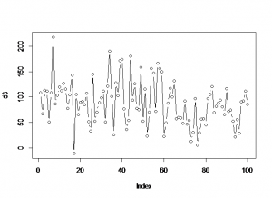
Generate a set of data where the distribution parameters change part way through:

d1<-rnorm(n,mean,sd)
d1<-rnorm(65,98,45)
d2<-rnorm(35,67,35)
d3<-c(d1,d2)
plot(d3,type="b")


The following table gives the distribution and the command for generating n data from each distribution.

Gaussian rnorm(n, mean=0, sd=1)
Exponential rexp(n, rate=1)
Gamma rgamma(n, shape, scale=1)
Poisson rpois(n, lambda)
Weibull rweibull(n, shape, scale=1)
Cauchy rcauchy(n, location=0, scale=1)
Beta rbeta(n, shape1, shape2)
'Student' (T) rt(n, df)
Fisher-Snedecor (F) rf(n, df1, df2)
Pearson (Chi-squared) rchisq(n, df)
Binomial rbinom(n, size, prob)
Multinomial rmultinom(n, size, prob)
Geometric rgeom(n, prob)
Hypergeometric rhyper(nn, m, n, k)
Logistic rlogis(n, location=0, scale=1)
Lognormal rlnorm(n, meanlog=0, sdlog=1)
Negative Binomial rnbinom(n, size, prob)
Uniform runif(n, min=0, max=1)
Wilcoxon's statistics rwilcox(nn, m, n), rsignrank(nn, n)