Correlation Matrix in R CRAN

Here it should be assumed that you have the values as columns on a spreadsheet and everywhere you don’t have a value you have replaced the gap with the letters NA.

Month A B C D E
Apr 63.91419 21.13823 75.13719 80.97858 11.86916
May 92.51104 126.4206 129.9751 56.79248 36.77565
Jun 65.44783 39.14822 6.558068 19.42456 21.63901
Jul 131.4266 70.55551 63.00389 102.5545 116
Aug 129.3926 31.60157 2.435477 NA 73.03078
Sep 35.71819 6.667624 89.68176 98.86681 26.59825
Oct 53.36333 97.32301 63.80283 2.39816 41.05988
Nov 38.88958 88.80514 118.4024 3.027732 64.32666
Dec NA 123.3156 123.5542 79.57653 62.26653
Jan 6.570292 11.66491 72.28813 31.43667 39.0891
Feb 15.1047 9.964003 144.4861 48.67408 146.2865
Mar 78.85201 10.53091 147.5341 67.90013 40.08176

Copy The Data into the clipboard:

cr<-read.table("clipboard",header=TRUE, na.strings="NA" )
x <-cr[2:5]
 cm<-cor(x,x,use = "pairwise.complete.obs")

Now output the Matrix back to the clipboard

write.table(cm,"clipboard",sep="\t")

and paste it back into Excel &c.

If you get a buffer full error then use :

write.table(cm,"clipboard-2048",sep="\t")

instead

A B C D
A 1 0.3 -0 0.4
B 0.3 1 0.2 -0
C -0 0.2 1 0.2
D 0.4 -0 0.2 1

Handy Packages for R

Packages:
lattice
envelope
doBy
RODBC
fArma
BayesX
car
maptools
RColorBrewer

install.packages("lattice", dependencies = TRUE)
install.packages("envelope", dependencies = TRUE)
install.packages("doBy", dependencies = TRUE)
install.packages("RODBC", dependencies = TRUE)
install.packages("fArma", dependencies = TRUE)
install.packages("BayesX", dependencies = TRUE)
install.packages("car", dependencies = TRUE)
install.packages("maptools", dependencies = TRUE)
install.packages("KernSmooth", dependencies = TRUE)
install.packages("RColorBrewer", dependencies = TRUE)

or in one command…

install.packages(c("rJava","lattice","Cairo","xlsx","treemap","RODBC","maptools","doBy","car","RColorBrewer","envelope","BayesX", "KernSmooth"), dependencies = T, repos = "http://cran.fhcrc.org") 

Generate Random data in R

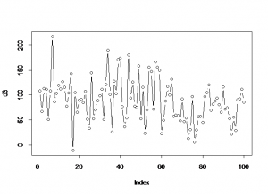
Generate a set of data where the distribution parameters change part way through:

d1<-rnorm(n,mean,sd)
d1<-rnorm(65,98,45)
d2<-rnorm(35,67,35)
d3<-c(d1,d2)
plot(d3,type="b")


The following table gives the distribution and the command for generating n data from each distribution.

Gaussian rnorm(n, mean=0, sd=1)
Exponential rexp(n, rate=1)
Gamma rgamma(n, shape, scale=1)
Poisson rpois(n, lambda)
Weibull rweibull(n, shape, scale=1)
Cauchy rcauchy(n, location=0, scale=1)
Beta rbeta(n, shape1, shape2)
'Student' (T) rt(n, df)
Fisher-Snedecor (F) rf(n, df1, df2)
Pearson (Chi-squared) rchisq(n, df)
Binomial rbinom(n, size, prob)
Multinomial rmultinom(n, size, prob)
Geometric rgeom(n, prob)
Hypergeometric rhyper(nn, m, n, k)
Logistic rlogis(n, location=0, scale=1)
Lognormal rlnorm(n, meanlog=0, sdlog=1)
Negative Binomial rnbinom(n, size, prob)
Uniform runif(n, min=0, max=1)
Wilcoxon's statistics rwilcox(nn, m, n), rsignrank(nn, n)

Automate an output using “while”

X<-2008
name<-"Flintshire"
maxY<-4500
while(X<2034){
png(paste("C:/PLOTS/",name, X ,".png"),width = 800, height = 600,units="px",bg="white")
plot(Persons~Age,data=subset(a,Area==name & Year==X), type='l', col="red", ylim=c(0,maxY)
,main=paste("Population Prediction: ",name," Year: ",X)
)
dev.off()
Y<-X
X<-Y+1}

once completed then animate using imagemagick

convert   -delay 20   -loop 0   Flintshire*.png   Flintshire.gif

and also some more:

#library(RODBC)
#library(lattice)

ch<-odbcConnect("cposerver")
sqlTables(ch)
c<-sqlQuery(ch, paste("select dttm ,count(*) as N" 
,"FROM MGW_AnE_BASE as a join DateTimeList as t on 1=1 and t.dttm between a.arrival_Dttm and depart_Dttm" 
,"GROUP BY t.dttm order by t.dttm")
)

str(c)

x1<-1
x2<-2016
for(j in 1:length(c$dttm)) {

png(paste("C:/PLOTS/PLOTS_", x1 ,".png")
,width = 1900, height = 600,units="px",bg="white")

plot(N ~ dttm
,data=subset(c, dttm >= c$dttm[x1] & dttm <= c$dttm[x2]) 
,type="l"
,ylim=c(0,50)
)

mtext(paste(x1))
dev.off()
x1<-x1+12
x2<-x2+12
}
dev.off()


Auto PNG of adjusted bi valued plot

##load the required bits
library(RODBC) ##for DB connection
library(doBy) ##for summaryBy
library(grDevices)## for outpur to PNG
channel<-odbcConnect("mike_db", uid="mike")
a<-sqlFetch(channel,"AnE_ind")
c<-summaryBy(wait~month_val,data=a, FUN=function(x){c(mean=mean(x),sd=sd(x),l=length(x),m=median(x))})
###########################
png(width = 750, height = 500,units="px",file="Z:/PLOTS/myplot3.png",bg="white")
par(mar=c(5, 4, 4, 5) + 0.1) ##add a margin to all subsequent charts
plot(
wait.l~month_val,data=c, type="l",lwd=1,col="blue"
,ylim=c(0,max(wait.l)+0) 
	, xlab="Date", ylab=""
	,main="YG Monthly A&E Attendance (Blue) 
	with Median Wait in minutes (Red)" 	)
par(new=T)
plot(wait.m~month_val,data=c,axes="F", type="l",lwd=1,ylim=c(0,max(wait.mean)+0)
,col="red",ylab="", xlab="")
mtext("Median Time Arrival to Discharge (mins)", col="red",4,2.4) ##"text", colour,side , offset
axis(side=4)
mtext("Monthly Attendance", col="blue",2,2.4)
axis(side=4)
dev.off()
########################################
ygts<-ts(c$wait.l,frequency=12)
plot(decompose(ygts))
########################################
ygMts<-ts(c$wait.m,frequency=12)
plot(decompose(ygMts))
########################################

sql access part 2 with boxplot and big query

##load the required bits
library(RODBC)
library(lattice)
##set up the connection
channel<-odbcConnect("mike_db", uid="mike")
##sqlTables(channel)
##a<-sqlFetch(channel,"AnE")
##b<-sqlFetch(channel,"vwAnE")
##b<-sqlQuery(channel, paste("select * from vwAnE order by loc, month_val"))
##xyplot(N~month_val|LOC,b, type="l")

##c<-sqlQuery(channel, paste("select CM,sum(numerator)"
##					,"from EP_2010_2011_ENHANCED"#
##					, "WHERE not parnt like 'z_%' "
##					," group by CM"
##					))

##execute a query for the data
e<-sqlQuery(channel, paste("select CM,aggregate_02,spect,Numerator,denominator,value,target, year_month+'-01' as year_month" 
,"from EP_2010_2011_ENHANCED"
,"where 1=1 and CM like '%e_01%'and TIME_TYPE='per-month'"
,"and parnt like 'z_t%'order by aggregate_02,spect,year_month"))
##convert the year_month value to a date

e$year_month<-as.Date(e$year_month)

##plot the lattice

xyplot(value~year_month|spect,e, type="l", cex=3)


xyplot(value+target~year_month|spect,e, type="l", size=5)